The goal of this article is to introduce another way to think about R0 (“R naught”, aka the basic reproduction number, a mathematical quantity that captures how contagious an infectious disease is) that doesn’t involve differential equations. When I first learned about it, I thought it was very interesting and highly applicable. This article assumes some basic knowledge of probability and Markov chains.
Since I study mathematics and not epidemiology, I can only give a brief mathematical introduction to the standard view of R0 here for completeness of this writing. I will then go into the actual focus of this article, which is a probabilistic and Markov Chain derivation of the basic reproduction number.
The SIR Model
In the compartmental SIR (susceptible-infected-removed) model, one derives this quantity by looking at the system of differential equations:
\frac{dS}{dt} = -\frac{\beta I S}{N}, \quad\quad\quad (1)\frac{dI}{dt} = \frac{\beta I S}{N} - v I, \quad\quad\quad (2)\frac{dR}{dt} = vI, \quad\quad\quad\quad (3)where S is the number of susceptible individuals in the population, I the number of infected individuals, and R recovered.
In Eq. (2) we see that the rate of change in the number of infected individuals is given by how fast new infections are occurring through contact with the already-infected individuals, minus how fast they are recovering (or dying). The number of infected people will grow if \frac{dI}{dt} > 0, that is,
\frac{\beta I S}{N} - vI> 0.At the beginning of a disease spread, without any additional information, it makes sense to assume that nearly everyone could be susceptible. With this assumption, \frac{S}{N} \approx 1. Replacing \frac{S}{N} with 1 gives
\frac{\beta}{v} := R_0 > 1,when the disease begins to take hold.
Note that without this assumption, we would obtain the effective reproduction number instead.
Now, another way we can think about R0 is by looking at a simple probabilistic model of cascade. In stochastic processes, it is often referred to as a branching process. This idea is not new by any means; researchers have used this model to study many kinds of things (spread of diseases, spread of ideologies online, births and deaths and survival of names and populations, etc).
A simple probabilistic model of cascade
To understand why the probabilistic component of this model might be useful, imagine that when an infected person goes out to interact with their contact network, there is a probability associated with whether or not they will spread the disease. Then, the people in that contact network who catch the disease can then spread it again to others in their respective contact network with some probability.
So let’s us consider a model with the 2 beginning assumptions:
- An infected individual (let’s call them Sam) on average has a contact network of size k individuals who Sam will meet independently,
- Sam transmits the disease to each of the k people with probability p.
And then let’s assume that these assumptions also hold for everyone else in that population.
In the first wave, Sam will meet k people. Then by our assumption each of those k people will meet k other people.
In the second wave, there would be k⋅k = k^2 individuals susceptible to secondary infections that started from Sam. And k^3 in the third wave, and so on.
We can visualize this branching process of the contact network as follows:
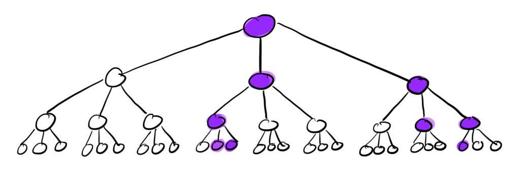
The purple nodes in this cascade tree with k=3 are the infected nodes. So after 3 waves with some value of p, we end up with 9 infected individuals starting from just 1.
Now, since each person who Sam meets in the first wave will be infected with probability p, we would on average have p \cdot k infected individuals. Then, in the second wave, these p \cdot k individuals will spread it to the k people that they meet, so on average the number of infected individuals after this wave would be
(p \cdot k)⋅p⋅k = (pk)^2.
If we repeat the process, we find that we expect to have (pk)^n infected individuals in the n-th wave. This quantity pk is our basic reproduction number.
Markov chains
More rigorously, let us turn to Markov chains to illustrate this. Let the random variable X_n be the number of infected individuals at time n (let’s assume we have discretized time into discrete steps so that time step n is equivalent to the n-th wave). (X_n) is a discrete time Markov chain since it satisfies the memoryless property: the number of infected people tomorrow only depends on the number of infected people today and no other information in the past is required.
By our assumptions, the expected number of secondary infections from one infected individual is
R_0 = \mathbb{E}[X_1|X_0=1] = \sum_{K=1}^{{\infty}} Kp_K = p_kk.To see this, note that p_K = 0 when K \neq k because by assumption one individual can only infect k different individuals independently with probability p ( = p_k).
So then,
\mathbb{E}[X_n|X_{n-1}] = R_0 \cdot X_{n-1}.Taking expectations again on both sides and using the law of total expectation,
\mathbb{E}[X_n] = R_0 \cdot \mathbb{E}[X_{n-1}] = R_0^n \cdot \mathbb{E}[X_0] = R_0^n,since X_0 = 1 (the only infected individual is Sam).
R_0 < 1 \implies E[X_n] \rightarrow 0 \text{ as } n \rightarrow \infty.In words, if R0 < 1, we expect that the number of infected individuals at time n will go to 0 when n is large with probability 1.
So now we see why it is important for diseases to have a basic (or effective) reproduction number less than 1 for it to have a possibility of dying out before infecting everyone.
Extinction Probability
But what if R0 > 1? Surely the larger the value, the worse it will get. But are we doomed? Not necessarily.
The question of whether there is there a positive probability that the disease will die out (so-called the extinction probability) is another thing that people can study, although this will be the topic of another time.